In order to help NetEase Cloud Music (NCM) enhance user experience and ultimately improve its user engagement, we aim to differentiate inactive users from active users and build a personalized recommender system. In this report we provide a summary of our findings from analysis of the NCM business case and the accompanying data set. The code used to perform the analysis and develop recommender systems can be found in my Github.
This report is structured around 4 main sections:
1. Introduction and Business Goals
- About NCM
- The Data
- Our Goals
2. User Characteristics and Engagement
A detailed analysis of the NCM dataset to produce insight and understanding regarding user characteristics and preferences.
- Usage Scenarios
- User Activity Intensity
- User Demographics: location, gender and age
- User Behavior and Preferences: tenure, impression and content
3. User Activity Prediction Model
Models to predict user activity based on users’ early actions.
- Logistic Regression
- SVM
- Random Forest
- Neural Networks
4. Recommender System
- A review of recommender system best practice
- Recommender systems for NCM and their relative merit and demerit
5. Business Implications
- Recommendations to NCM
This post contains Section 3. Please check here for section 1 and 2, and here for Section 4 and 5.
3. User Activity Prediction Model
The code for this section is available here: Appendix II.
As evident from the user characteristics in the previous sections(see Part I), there is a ‘hub-and-tail’ type distribution when it comes to the activity levels of the users and popularity of content, i.e., there are a few highly active users and viral cards, and many middle to low activity users and low popularity content. This kind of distribution, also known as a Power Law Distribution, is very commonly seen in various aspects of social networks and is one of the roadblocks when it comes to setting up successful predictive models on social data (Muchnik, L., Pei, S., Parra, L. et al.,2013). Predictive models are additionally difficult because of factors like (i) user diversity – wherein a global model may not be applicable to all users, (ii) social influence – as user relationships can greatly influence activity and (iii) the dynamic nature of such networks where user behaviour can easily change over time (Zhu Y., Zhong E., Pan S.J., et.al, 2013).
Despite these obstacles, there is great inherent commercial value predicting the behaviour of a user. In the case of NCM , marketing and recommendation strategies can be more focused and differentiated for active vs. non-active users based on different desired end goals, resulting in reduced costs. With this motivation in mind, we looked to apply machine learning models and methodologies to predict whether a user will be active or inactive in the future based on their early actions.
3.1 Model Preparation
To set up the model, the individual impression level data from the ‘impression_data’ file (with 30 days of records) was grouped by ‘userId’ and the values transformed as below to get our desired input and target variables:
- The first 10 days of data (‘dt’ <= 10) for each user is summed up to get 13 input variables, i.e., the summed activity of each user in the first 10 days including card impressions, clicks, comments, into personal homepage, shares, view comment, likes, view time and the demographic information of each user including province, age, gender, egistered months and total number of accounts followed.
- The remaining days of data for each user are transformed into the target variable under the same condition discussed earlier, now applied to the 20 day timeline, to achieve a binary output variable with 1 indicating future active users and 0 indicating future inactive users. In mathematical terms, for each user i, the below transformation is applied:
Hence, the goal of our predictive model is a binary classification of users into future active or future inactive based on the initial 10 days of data, with our class of interest being future active users and our goal being finding out the model with best performance. Common machine learning models for binary classification are Logistic Regression and Support Vector Machines (SVM), and hence they are our first choices to test out. We also look at Random Forest as they are purportedly apt for general classification problems, and Neural Networks (NN) as they can result in high levels of accuracy but at the cost of interpretability.
Additionally, there are some important aspects of this predictive problem that need to be taken into consideration before implementing the models.
- Firstly, it is noted that our dataset is somewhat imbalanced i.e., the number of active users is much smaller (represents only about 22% of total users in the dataset for prediction models). To increase the generalizability of our models and recall for the class of interest, we utilize the upsampling technique, applying 4 times random sampling among active users within the same sample dataset to increase the active users size. As a result, the data size in the new dataset increase from 628,788 to 1,188,448, with around 47% active users.
- Secondly, there are plenty null value in the ‘mlogViewTime’ column in impression dataset and ‘age’ and ‘gender’ column in user_demographic dataset. We assign zero to null value in ‘mlogViewTime’ under the assumption that missing data implied no views and browsing streams. We also replace null value in ‘age’ with zero, so that it could represent a single group itself, instead of assigning a mean or median value which would fall into the existing age groups. For null value in ‘gender’, we simply replace them with ‘unknown’.
- Thirdly, the categorical variables ‘province’ and ‘gender’ are tranfered into dummy variables as dummy variables allows easy interpretation and calculation of the odds ratios, and increases the stability and significance of the coefficients (Garavaglia,et.al, 1998). And we scale the numerical variables by Z-score normalization, bringing all features in the same standing, so that one significant feature doesn’t impact the model just because of its large magnitude.
- Lastly, we have a very large dataset, posing various technical challenges on top of the complexity of the algorithms at hand. For example, the complexity of SVM with nonlinear-kernels is approximately $O(n_samples^2 * n_features)$. With our dataset, it takes forever for a personal laptop to get results. Therefore, for simplicity, we take randomly 10% of the data as a sample to train the models. Further methods of sample selection can be done to improve accuracy, such as instance selection.
Next, several machine learning models are applied, including Logistics Regression, SVM, Random Forest and Neural Networks. We shuffle and split the data to 60% training set, 20% validation set and 20% test set. For Logistics Regression, SVM and Random Forest, we use Grid Search Cross-Validation to get the optimal setting of hyperparameters. For Neural Networks, we do hyperparameters tuning on training set and use the validation set to select the best hyperparameters(Jason Brownlee, 2019). We then use test set to evaluate the model performance using accuracy score and mean squared error, and compute its confusion matrix and classification report.
3.2 Logistics Regression
Logistic regression is a popular machine learning algorithm for supervised classification problems, which is often used as a baseline model. It assumes that the classes are almost or perfectly linearly seperable. Here we have a binary logistic regression model with 2 possible outcomes, i.e., 1 for active and 0 for inactive. Data is fitted into a linear regression model which then be squashed within the range [0, 1] by a logistic function. If the squashed value is greater than a threshold value(0.5), we assign it a label 1, else we assign it a label 0.
Hyperparameters Tuning
Hyperparameters
-
Solver:
Saga is an extension of sag that also allows for L1 regularization and it should generally train faster than sag. And newton-cg is slow for large datasets, because it computes the second derivatives. Therefore, we exclude sag and newton-cg in our solver test set. -
Penalty:
L1, L2 and no penalty -
C (inverse of regularization strength):
A high value of C tells the model to give high weight to the training data, and a lower weight to the complexity penalty. A low value tells the model to give more weight to this complexity penalty at the expense of fitting to the training data. Here we will try C = 100, 10, 1.0, 0.1 and 0.01.
Tuning Technique
We use Grid Search Cross-Validation instead of Train-Validation-Test to select the best model, parameterized by a grid of hyperparameters.
Model and Performance
The optimal hyperparameters we get from Grid Search is C = 0.01, penalty = L1 and solver = saga. After retraining the model with the best setting of hyperparameters and apply the optimal logistic regression to the test set, we get the following results:
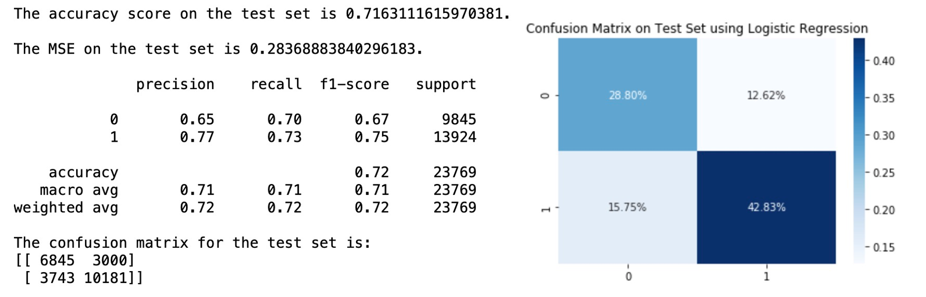
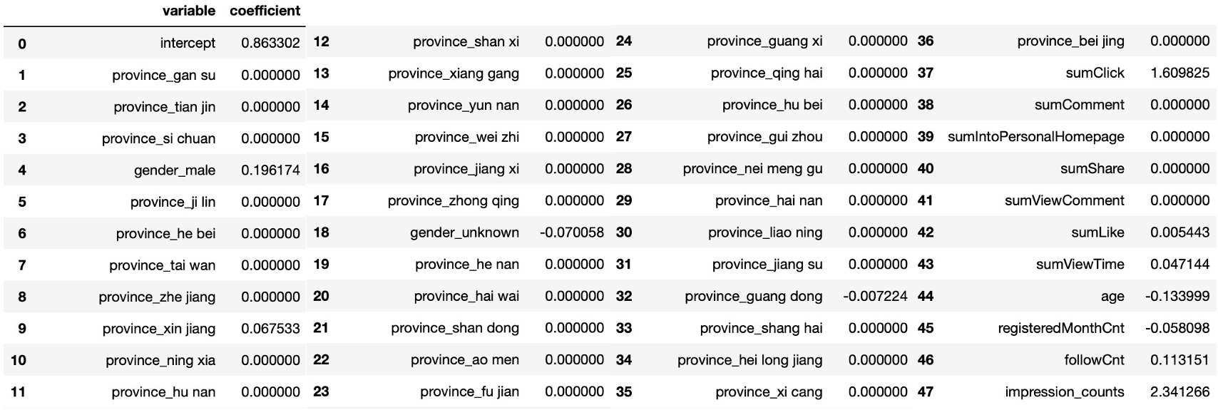
The accuracy score on test set is about 0.7202, and the accuracy score for our class of interest (active user) is higher than that of the inactive class. From the coefficient table above, we can find that sum of clicks and impressions have the largest magnitude of positive impact, implying that these actions are the most characteristic of active users. The variables registeredMonthCnt and age however show a negative impact but relatively small in magnitude. These are in line with our findings in the previous sections.
3.3 SVM
Support Vector Machine is another popular supervised learning algorithm which can be used for classification and regression problems as support vector classification (SVC) and support vector regression (SVR). The objective of the support vector machine algorithm is to find a hyperplane with the maximum margin in an N-dimensional space(N is the number of features) that distinctly classifies the data points. In case of non-linearly separable data, Kernelized SVM is used instead of the simple SVM.
Hyperparameters Tuning
Hyperparameters
-
Kernel(control the manner in which the input variables will be projected):
Linear: A linear kernel can be used as normal dot product any two given observations. The product between two vectors is the sum of the multiplication of each pair of input values. It proves to be the best function when there are lots of features.
Polynomial: A polynomial kernel is a more generalized form of the linear kernel. The polynomial kernel can distinguish curved or nonlinear input space.
Radial Basis Function Kernel: RBF can map an input space in infinite dimensional space. It is usually chosen for non-linear data.
Sigmoid:It is mostly preferred for neural networks. This kernel function is similar to a two-layer perceptron model of the neural network, which works as an activation function for neurons. We will not implement the ‘sigmoid’ kernel here as it is essentially a proxy for neural networks which we will be looking at separately later. -
C (regularization parameter):
This is how you can control the trade-off between decision boundary and misclassification term. A smaller value of C creates a larger-margin hyperplane and a larger value of C creates a smaller-margin hyperplane. Here we will try C = 100, 10, 1.0, 0.1 and 0.01. -
Gamma:
Kernel coefficient for ‘rbf’, ‘poly’ and ‘sigmoid’. It defines how far the influence of a single training example reaches, with low values meaning ‘far’ and high values meaning ‘close’. We will use the default setting in sklearn which is ‘scale’, i.e., gamma = 1 / (n_features * X.var())
Tuning Technique
We use Grid Search Cross-Validation instead of Train-Validation-Test to select the best model, parameterized by a grid of hyperparameters.
Model and Performance
The optimal hyperparameters we get from Grid Search is C = 100, kernel = ‘rbf’ and gamma = ‘scale’. After retraining the model with the best setting of hyperparameters and apply the optimal SVM to the test set, we get the following results:
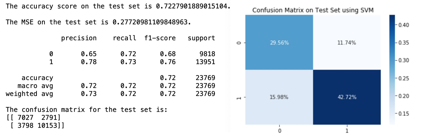
The accuracy score on test set is about 0.7228, and the accuracy score for our class of interest (active user) is higher than that of the inactive class.
3.4 Random Forest
Random Forest is a supervised machine learning algorithm that can be used to solve regression and classification problems. It utilizes ensemble learning that combines many classifiers to provide solutions to complex problems. Random forest involves constructing a large number of decision trees from bootstrap samples from the training dataset, like bagging. But random forest also involves selecting a subset of input features at each split point in the construction of trees which is better than bagging. By reducing the features to a random subset that may be considered at each split point, it forces each decision tree in the ensemble to be more different and these less correlated trees are averaged to make a prediction, which often results in better performance than bagged decision trees.(Page 320, An Introduction to Statistical Learning with Applications in R, 2014)
Hyperparameters Tuning
Hyperparameters
-
max_features
The most important hyperparameter to tune for the random forest is the number of random features to consider at each split point. A good heuristic for classification is to set this hyperparameter to the square root of the number of input features.(Page 387, Applied Predictive Modeling, 2013)
num_features_for_split = sqrt(total_input_features) -
max_depth
Another important hyperparameter to tune is the depth of the decision trees. Deeper trees are often more overfit to the training data, but also less correlated, which in turn may improve the performance of the ensemble. Depths from 1 to 10 levels may be effective. -
n_estimators
Ideally, this should be increased until no further improvement is seen in the model. Good values might be a log scale from 10 to 1,000.
Tuning Technique
We use Grid Search Cross-Validation instead of Train-Validation-Test to select the best model, parameterized by a grid of hyperparameters.
Model and Performance
The optimal hyperparameters we get from Grid Search is max_depth = 10, max_features = ‘sqrt’ and n_estimators = 1000. After retraining the model with the best setting of hyperparameters and apply the optimal Random Forest to the test set, we get the following results:
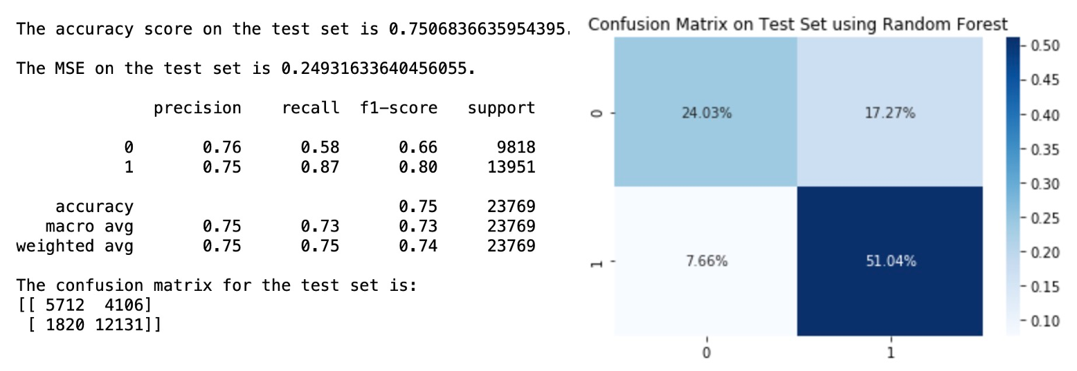
The accuracy score on test set is about 0.7507, and the accuracy score for our class of interest (active user) is higher than that of the inactive class. And we can see that the there are less false negative cases in Random Forest compared with SVM and Logistic Regression.
3.5 Neural Networks
Neural networks are multi-layer networks of neurons that we use to make classification and predictions which can either be supervised or unsupervised. Here is a brief and clear introduction of Neural Networks from Tony Yiu, which I think is a very good reading to understand the basics of this algorithm. His opinion about the aspects that make Neural Networks special can be summarized as:
(i) Each neuron is its own miniature model with its own bias and set of incoming features and weights. (ii) Each individual model/neuron feeds into numerous other individual neurons across all the hidden layers of the model. So we end up with models plugged into other models in a way where the sum is greater than its parts. This allows neural networks to fit all the nooks and crannies of our data including the nonlinear parts (but beware overfitting — and definitely consider regularization to protect your model from underperforming when confronted with new and out of sample data). (iii) The versatility of the many interconnected models approach and the ability of the backpropagation process to efficiently and optimally set the weights and biases of each model lets the neural network to robustly “learn” from data in ways that many other algorithms cannot.
After understanding how this algorithm works, we start to tune hyperparatmers.
Hyperparameters Tuning
Hyperparameters
When forming the model, there are two decisions that must be made regarding the hidden layers:
-
How many hidden layers to actually have in the Neural Networks?
(i) If the data is linearly separable then you don’t need any hidden layers at all.
(ii) If data is less complex and is having fewer dimensions or features then neural networks with 1 to 2 hidden layers would work.
(iii) If data is having large dimensions or features then to get an optimum solution, 3 to 5 hidden layers can be used.
In our case, we have the 47 inputs which is relatively large, 3 to 5 hidden layers are more suitable. But increasing hidden layers will also increase the complexity of the model, as the rationale behind the building of the first NN model trained is to keep it as simple as possibleso, we will choose 3 here which is the smallest among 3,4,5. -
How many neurons will be in each of these layers?
(i) Input layer: the input layer will consist of 47 neurons.
(ii) Output layer: the output layer will have 2 neurons, one per class.
(iii) Hidden layer: when deciding the number of neurons on hidden layers, we can consider the following rules: The number of hidden neurons should be between the size of the input layer and the output layer. The most appropriate number of hidden neurons is sqrt(input layer nodes * output layer nodes). The number of hidden neurons should keep on decreasing in subsequent layers to get more and more close to pattern and feature extraction and to identify the target class.
According to these rules, we can get that the number of hidden neurons is between 2 and 47 and the most appropriate number of hidden neurons is sqrt(2*47) ≈ 10. We will set the number of neurons on the middle hidden layer as 10 and we choose 28 (which is in the middle of 47 and 10) and 6 (which is in the middle of 10 and 2) neurons for the first and third hidden layers.
Above all, we are going to set in total 5 layers, including an input layer with 47 neurons, 3 hidden layers with 28, 10 and 6 hidden neurons on each layer. The hidden layers employs the standard ‘ReLu’ activation function, while for the final layer as we had a binary classification task the ‘sigmoid’ function is used.
In terms of the loss, we adopt the ‘SparseCategoricalCrossentropy’ function as it produces a category index of the most likely matching category which can save space and also match with the format of our output. And we use the ‘adam’ version of the stochastic gradient descent algorithm to minimize losses.
Then we will change the epochs and batch size in the fit function.
-
The batch size is a number of samples processed before the model is updated. When all training samples are used to create one batch, the learning algorithm is called batch gradient descent. When the batch is the size of one sample, the learning algorithm is called stochastic gradient descent. When the batch size is more than one sample and less than the size of the training dataset, the learning algorithm is called mini-batch gradient descent. In the case of mini-batch gradient descent, popular batch sizes include 32, 64, and 128 samples.
-
The number of epochs is the number of complete passes through the training dataset. The number of epochs can be set to an integer value between one and infinity. You may see examples of the number of epochs in the literature and in tutorials set to 10, 100, 500, 1000, and larger.
Here, we will try stochastic gradient descent with batch size 1. And 3 different epochs which are 10, 100 and 1000.
Tuning Technique
We will apply the training-validation-test procedure to find out the best value for epochs.
Model and Performance
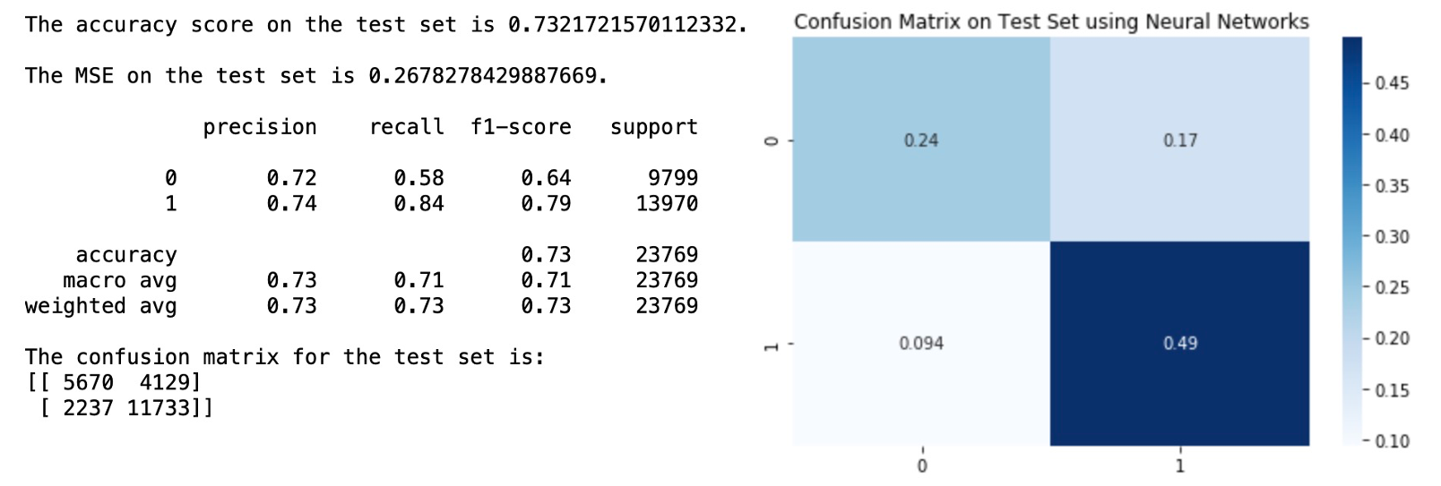
The accuracy score on test set is about 0.7322, and the accuracy score for our class of interest (active user) is higher than that of the inactive class.
3.6 Final Activity Prediction Model & Results
The accuracy of above candidate models are summarized below:
| Accuracy | Precision | Recall | F1-score | |
|---|---|---|---|---|
| Logistic Regression | 0.7163 | 0.71 | 0.71 | 0.71 |
| SVM | 0.7228 | 0.72 | 0.72 | 0.72 |
| Random Forest | 0.7507 | 0.75 | 0.73 | 0.73 |
| Neural Networks | 0.7322 | 0.73 | 0.71 | 0.71 |
We select the Random Forest with upsampling as our final chosen prediction model for the following reasons:
It has the highest accuracy score, as well as precision, recall and f1-score. And it shows the least false negative cases among all the candidate models. For NCM, predicting future active users correctly (and minimizing false negatives) would be of utmost commercial importance as they can target them accordingly to strategically build their user base and minimize the opportunity cost of losing incorrectly targeted future active users.
Still, the accuracy score of our selected model is not high enough. Some of the improvements we suggest moving forward would be to enable lifting the constraints faced by the current modelling environment, such as:
- acquiring more computing power to train the model on more data,
- obtaining data over a longer time period,
- adding in social network features such as connections and relationships,
- as well as potentially structurally changing the problem into a multiclass one with activity level labels instead, based on a more sophisticated user activity criterion (this would require a different choice of base model).
Thus, our selected final model provides a springboard based on which more advanced modeling and tuning can be conducted, given additional resources, to achieve increased accuracy metrics.
References
-
Garavaglia, S.B., Dun, A.S., & Hill, B.M. (1998). A smart guide to dummy variables: four applications and a macro.
-
Jason Brownlee. (2019). Tune Hyperparameters for Classification Machine Learning Algorithms. Available from: https://machinelearningmastery.com/hyperparameters-for-classification-machine-learning-algorithms/
-
Muchnik, L., Pei, S., Parra, L. et al. (2013) Origins of power-law degree distribution in the heterogeneity of human activity in social networks. Sci Rep 3, 1783. Available from: https://doi.org/10.1038/srep01783
-
Zhang, D., Hu, M., Liu, X., Wu, Y., & Li, Y. (2020). NetEase Cloud Music Data. Manufacturing & Service Operations Management.
-
Zhu Y., Zhong E., Pan S.J., et.al. (2013). Predicting user activity level in social networks. Proceedings of the 22nd ACM international conference on Information & Knowledge Management (CIKM ‘13). Association for Computing Machinery, New York, NY, USA, 159–168. Available from: https://doi.org/10.1145/2505515.2505518